5 Artificial Neural Network
5.1 Introduction
Artificial Neural Networks (ANN) are a family of computational systems capable of machine learning and pattern recognition based on biological nervous systems (for example the animal brain) (see figure 5.1). The main applications of ANNs involve computer vision, machine translation, social network filtering, speech recognition and medical diagnosis.
![A biological neural network (left) and an artificial neural network (right) *[Source: @R-makinde]*](Images/ann.png)
Figure 5.1: A biological neural network (left) and an artificial neural network (right) (Source: Makinde and Asuquo 2012)
ANN has increasingly draws attention within the industry and the academia (for a detailed presentation of ANN, see Zafeiris and Ball (2018) and also Wang and Zhong (2016)).
5.2 Method Description
Typical ANNs models have a novel structure. In this structure, artificial neurons are aggregated into layers (figure 5.2). The input layer is the leftmost, the hidden layer stands in the middle and the output layer is on the right of the network. The neural network is composed of a number of nodes (the neurons) and weighted connections between the nodes (the synapses).
Nodes called artificial neurons in the neural network can range from several to thousands depending on the complexity of the task to achieve. Similarly, the neural network can have a single hidden layer or multiple hidden layers depending on the task. In a neural network, a signal is transmitted from one node to another. The signal received by a node is processed and then signals additional nodes connected to it. This is known as multilayer feed-forward network, where each layer of nodes receives inputs from the previous layer.
The input layer contains nodes, variables that encoded the values used to predict an output. The hidden layer contains nodes that do the calculation on the signal passed from the input node and pass the result to the output node(s). In a multiple hidden layer network, the signal is passed to more than one hidden layer before being passed to the output node. The output node is the variable(s) that we intend to predict.
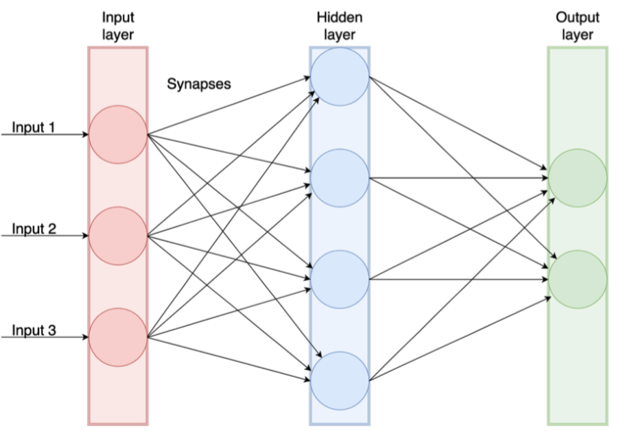
Figure 5.2: Sketch of a feed-forward artificial neural network
The hidden neuron is responsible for the calculation of the weighted of all the inputs (a weighted linear combination), adds a bias and then decides whether to fire a neuron sending the signal along the axon (figures 5.2 and 5.3). At each connection, called synapses or edge, between nodes, the transmitted signal will correspond to a real number (Gerven and Bohte 2018). This number is denominated weight and the learning process can be carried-on.
The increase or decrease of this weight influences the strength of the signal at the connection. The inputs to each node are aggregated using a weight linear combination (an analytical method applied when more than one attribute is taken into account). If the summation of equation (5.1) at the node is greater than a certain threshold value, the node transmits a signal along the axon to the next nodes connected to it. The output of each artificial neuron is modified by a non-linear function of the weighted sum of its inputs plus a bias (figure 5.3).
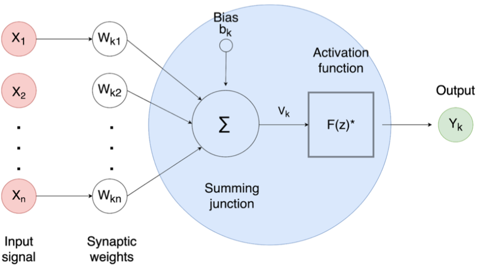
Figure 5.3: Sketch map of operations inside the hidden neuron
In equation (5.1), the parameters \(b_1, b_2, b_3\) and \(w_{1,1}, ..., w_{4,3}\) are “learned” from the data. The values of the weights are often restricted to prevent them from becoming too large. The parameter that restricts the weights is known as the decay parameter and is often set to be equal to 0.1.
In the hidden layer, these non-linear functions or activation functions, like the sigmoid function in (5.2), are used to complete the transformation from input nodes to an output layer. This transformation is carried out to reduce the effects of extreme input values making the network more robust and less susceptible to outliers.
\[\begin{equation} \text s(z) ={\frac {1}{1+e^-z}} \tag{5.2} \end{equation}\]The weights take random values to begin with, and these are then updated using the observed data. The network is usually trained several times using different random starting points, and the results are averaged. The number of hidden layers, and the number of nodes in each hidden layer, must be specified in advance.
ANN uses several models such as feed-forward and feedback propagation for prediction. Information moves on single direction for feed-forward network with no cycles or loops in the network. Supervised learning is employed in feedback propagation, requiring training data for predictive analysis. Figure 5.4 illustrates a standard process for ANN. The input data is used to training and testing procedures. After applying the model, the accuracy assessment must be done to evaluate the model.
![ANN modelling framework *[Source: @R-qazi]*](Images/annframework.png)
Figure 5.4: ANN modelling framework (Source: Qazi and Khan 2015)
5.3 The Modeling and Solving Approach
In this forecasting experiment, we will use supervised learning to train the dataset. As already mentioned in this book, supervised learning is applied by giving a set of labelled training data to the algorithm to predict labels for unseen data. This is achieved by first dividing the dataset into training and test using a 80%:20% ratio.
The first step we need to take prior to any command is to load the data to the space environement and to install some required packages.
There are several ANN libraries in R. The commonly used ones are amore, rsnns, neuralnet and nnet, the most widely used general purpose library for neural network analysis15
# install if necessary using 'install.packages'
# we will use a function from github
library(nnet)
source_url('https://gist.githubusercontent.com/fawda123/7471137/raw/466c1474d0a505ff044412703516c34f1a4684a5/nnet_plot_update.r')

# also, load the data to the space environement
load("forecasting.RData")
tts <- read_excel("tts.xlsx",
                  sheet = "transpose", col_names = FALSE)
In this chapter, the same procedure of the former exercises will be applied: 23 days as training data and 7 days as testing. Also, we will apply the feed-forward model, wherein connections between the nodes do not form a cycle, a different approach to recurrent neural networks. In this model, ANNs allow signals to travel one way only: from input to output. There are no feedback (loops), that means that the output of any layer does not affect that same layer. Feed-forward ANNs tend to be straightforward networks that associate inputs with outputs. They are extensively used in pattern recognition.16
In the experiment, the training data has to be split into two separate datasets so that we can use the previous 5-minute interval values to predict the next interval. A multiple-input and multiple-output ANN structure have to be deployed using the previous 5-minute interval for the unit travel time (UTT) values for all road links. This process is iterated so as to obtain 4140 observations which is the equivalent to 23 days split at a 5-minute interval.
UJT.chosen <- UJT[ ,c("1745","1882","1622","1412","1413","1419","2090","2054","2112",
                      "2357","2364","2059","2061","2062")]

# Divide dataset into training and testing data
training <- UJT.chosen[1:4140,]
testing <- UJT.chosen[4141:5400,]
training_1 <-training[-1,]
The following step after training the data involves setting the best tune parameters to carry out the prediction. The parameters that mut be set are: 1. decay (the weight decay) and 2. size (the number of neurons in the hidden layer). In this exercise, we will use a single hidden layer.
To ensure we get a good model, it is wise to test a range of values of each of the model parameters. To do this we will use the caret package. mygrid is the selection of parameters that will be tested. To optimize the parameters, a grid (expanded grid) with a set of decay and size values ranging from 5e-06 to 5e-01 and 1 to 10, are defined. Moreover, we are going to set a 10-fold cross-validation repeated 3 times. All this process must be carried-out to find the optimal model parameter (the decay and size) to be applied.
set.seed(6)
mygrid <- expand.grid(.decay=c(0.000005,0.00005,0.0005,0.005,0.05,0.5), .size=c(1:10))
fitControl <- trainControl("repeatedcv", number = 10, repeats = 3, returnResamp = "all")
set.seed(6)
nnet.parameters <- train(training[1:4139,1:14], training_1[,14], method = "nnet", metric = "log", trControl = fitControl, tuneGrid=mygrid)plot(nnet.parameters)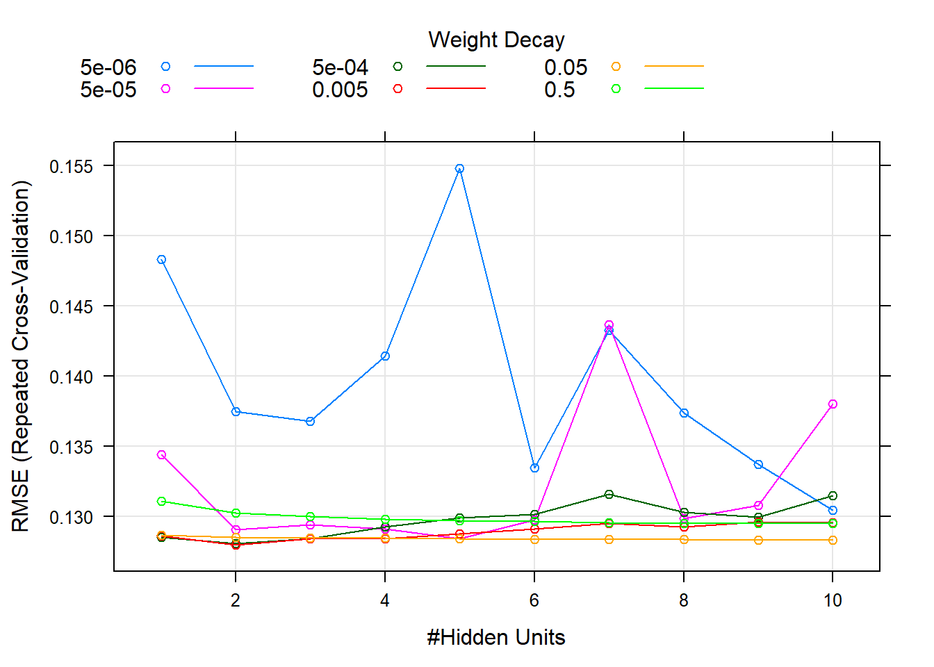
Figure 5.5: RMSE error in the traing data simulation using different size and decay parameters
Figure 5.5 displays the results of this process showing the change in error (RMSE) for the different weight decay and size (#Hidden Units). The same figure also reveals that weight 5e-03 and size 7 are the best-tunned parameters for this model.
The final step involves the prediction and validation of the model using unseen testing dataset. The prediction can be obtained using the best-tuned parameter as mentioned. Figure 5.6 presents the internal structure of the neural network using the best-tuned parameters.
Once the prediction for all the road links has been carried on, we must validate the model by assessing the observed results with the predicted ones. This is done comparing the mean absolute percent error (MAPE) and the mean square error (MSE) index generated between the predict values and observed values.
plot.nnet(nnet.parameters$finalModel)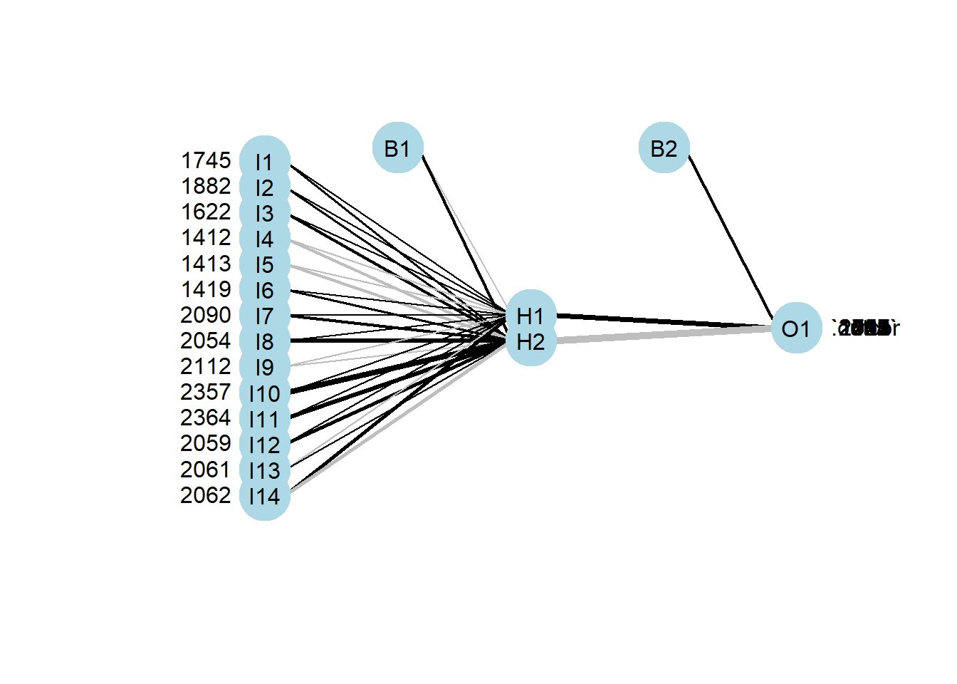
Figure 5.6: Internal structure of the ANN using the best-tuned parameters.
# Predict using best tune parameters
set.seed(6)
temp.nnet <- nnet(training[1:3960,], training_1[1:3960,], decay=5e-3, linout = TRUE, size=7)
set.seed(6)
temp.pred<-predict(temp.nnet, testing)
Here the decay parameter refers to the weight decay, the linout parameter switches to linear output units, and as our task is to do regression this parameter should be TRUE (the alternative is logistic units for classification). The size parameter refers to the number of neurons in the hidden layer. To look at the parameters you can control in nnet, consult the documentation using ?nnet on the console panel.
We finally can analyse the exercise results. Figure 5.7 displays the fit result for road link 2087.
We can note that the RMSE error for road links 473 and 2061 higher were higher (i.e. 0.07 and 0.11 in turns) compared to RMSE errors in road links 2087 and 2112, 0.02 and 0.04 respectively. This is also consistent with the MAPE errors values generated by the four-road links. MAPE errors in road links 473 and 2061 were also higher compared to road link 2087 and 2112. This means that road links 2087 and 2112 are more forecastable compared to road links 473 and 2061.
matplot(cbind(testing[,1], temp.pred[,1]),ylab="UTT", xlab="Lags", main="Road link 2087", type="l", lty = c(1,1), col = c("blue","red"))
legend(1,.35, legend = c("Test","Prediction"), lty = c(1,1), col = c("blue","red"),box.lwd = .5, cex = .65 )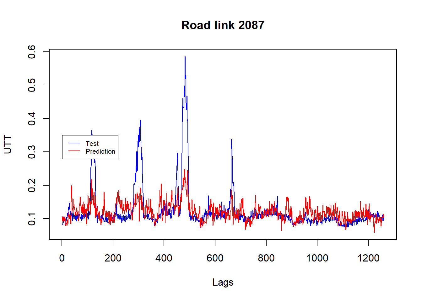
Figure 5.7: Observed versus forecast values for road link 2087 for 5-minute interval
5.4 Chapter Summary
This chapter introduced ANNs for time series modelling. Artificial neural networks are forecasting methods that are based on simple mathematical models of the brain. ANNs has shown to be very appropriated tool in many applications that involve dealing with complex real world sensor data.
A common criticism of neural networks, particularly in robotics, is that they require too much training for real-world operation. Nonetheless, because of their ability to reproduce and model nonlinear processes, artificial neural networks have found many applications in a wide range of disciplines such as system identification and control (vehicle control or trajectory prediction), quantum chemistry, general game playing, face identification and data mining.
References
Gerven, M., and S. (Eds.) Bohte. 2018. Artificial Neural Networks as Models of Neural Information Processing. Frontiers Media SA.
Makinde, Ako, F. A., and I. U. Asuquo. 2012. “Prediction of Crude Oil Viscosity Using Feed-Forward Back-Propagation Neural Network.” Petroleum & Coal 54: 120–31.
Qazi, Fayaz, A., and W.A. Khan. 2015. “The Artificial Neural Network for Solar Radiation Prediction and Designing Solar Systems: A Systematic Literature Review.” Journal of Cleaner Production 104: 1–12.
Wang, Tsapakis, J., and C. Zhong. 2016. “A Space–time Delay Neural Network Model for Travel Time Prediction.” Engineering Applications of Artificial Intelligence 52: 145–60.
Zafeiris, Rutella, D., and G. R. Ball. 2018. “An Artificial Neural Network Integrated Pipeline for Biomarker Discovery Using Alzheimer’s Disease as a Case Study.” Computational and Structural Biotechnology Journal 16: 77–87.
Package documentation is available at: http://www.rdocumentation.org/packages/nnet/versions/7.3-12/topics/nnet↩
This type of organisation is also referred to as bottom-up or top-down.↩