3 Seasonal and Trend Decomposition with Loess Forecasting Model (STLF)
3.1 Introduction
In Chapter 2, we see that parametric models describe the functional form of the relationship between the dependent and independent variables. It is not unusual for time series data to exhibit some type of upward or downward tendency over time, like trend and seasonability.
Time series comprise three eseential components: 1. a trend-cycle component, 2. a seasonal component and 3. a remainder component (containing anything else in the time series). When we decompose a time series into components, we usually combine the trend and cycle into a single trend-cycle component.
In this chapter, we will consider some common methods for extracting these components from a time series. Often this is done to help improve understanding of the time series, but it might also be used to improve forecast accuracy. It is important to mention that given the weak spatio-temporal autocorrelation (previoulsly examined in chapter 2) and the strong temporal autocorrelation on the LCAP network, the use of a local regression model does not require the series to be stationary, in contrast to ARIMA and Box-Jenkins approaches.
The STLF model is applied to time series decomposition with a non-seasonal forecasting method and was developed by (Cleveland and Terpenning 1990). In this chapter, we will apply the method to the data previously examined and select some road links to carry-on the method.
3.2 Method Description
The seasonal-trend decomposition with Loess (STLF) is a method for decomposing time series into: a seasonal component \(S_t\), a trend-cycle or simply trend component \(T_t\), and the reminder or error component \(R_t\) (Cleveland and Terpenning 1990). This decomposition may be additive (3.1) or multiplicative (3.2) where \(y_t\) is the data. A seasonally adjusted series is the result of removing the seasonal component from the data.
\[\begin{equation} \operatorname {y_t} = S_t + T_t + R_t \tag{3.1} \end{equation}\] \[\begin{equation} \operatorname {y_t} = S_t \times T_t \times R_t \tag{3.2} \end{equation}\]The method known as exponential smoothing state space model (ETS) is applied to algorithms which generate point forecasts to define prediction (or forecast) intervals.
ETS is able to generate a complete forecast distribution from an univariate time series using exponentially decaying weighted averages of past observations. The state space models correspond to the equations that describe how the error, trend, and seasonal components vary over time. Each of them can be categorised as additive (A), multiplicative (M), or none (N) (Hyndman and Athanasopoulos 2018). For example, ETS (A,N,N) represents a simple exponential smoothing with additive errors method and ETS (M,A,N) a Holt’s linear method with multiplicative errors (Holt 2004).
Putting them together, the STLF model applies a decomposition to a time series. It then models the seasonally adjusted series with an ETS method, re- seasonalizes the result, and finally returns the predictions or forecasts.
3.3 The Modeling and Solving Approach
To apply the model, we will divide the data as follows: the training set contains the UTT data for the first 23 days and the testing set considers the remaining 7 days. As previously described, there are 180 observations per day, one very 5 minutes from 6am to 9pm.
It is important to note that the model accounts only for temporal characteristics and no difference is going to be considered if the road links are adjacent on non-adjacent.
To set up the experience, first load tha data into the space environement as well as the required packages.
# set the working directory accordingly with setwd()
# load the data to the space environement
load("wksp2404.RData")

# install if necessary using 'install.packages'
library(grid)
library(ggplot2)
library(forecast)
library(grid)
In this experiment, four roads links have been randomly selected: IDs. 2112, 2087, 2061 and 473.
First, we will analyse the time series pattern of each road link. A daily pattern can be observed for road IDs 2112 and 2087 as displayed in Figure 3.1. We can also observe that the same pattern is not apparent for the first 2 roads because of large UTT values that can reach up to 8 seconds per metre.
# calculate UTT time series
p1 <- autoplot(ts_roadLink.2061, xlab ="Days", ylab="UTT 2061")
p1 <- p1 + theme(text = element_text(size = 15))
p2 <- autoplot(ts_roadLink.473, xlab ="Days", ylab="UTT 473")
p2 <- p2 + theme(text = element_text(size = 15))
p3 <- autoplot(ts_roadLink.2112, xlab ="Days", ylab="UTT 2112")
p3 <- p3 + theme(text = element_text(size = 15))
p4 <- autoplot(ts_roadLink.2087, xlab ="Days", ylab="UTT 2087")
p4 <- p4 + theme(text = element_text(size = 15))

# plot the results
grid.newpage()
grid.draw(rbind(ggplotGrob(p1),
                ggplotGrob(p2),
                ggplotGrob(p3),
                ggplotGrob(p4),
                size = "last"))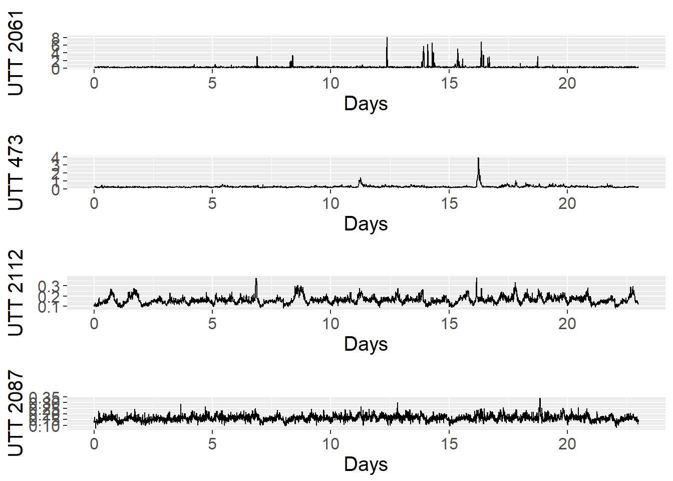
Figure 3.1: Training data set: UTT time series (23 first days) of 4 links
A polar plot displays a plot of radial lines, symbols or a polygon centered at the midpoint of the plot frame on a 0:360 circle. Positions are interpreted from the right and moving counterclockwise (clockwise is TRUE) unless specifying another starting point. If add = TRUE is passed as one of the additional arguments, the values will be added to the current plot. Figure 3.2 presents polar charts of UTT for the first 3 days of road links 2061 and 473.
A pattern can be observed between the different days (01/01/2011 - 03/01/2011), so a seasonal trend can be assumed for these road links as well.
# Define polar plot
ts_seasonplot = ts(training[1:540,"2061"],
                      start=0,
                      frequency=180)
ts_seasonplot2 = ts(training[1:540,"473"],
                   start=0,
                   frequency=180)
p1 <- ggseasonplot(ts_seasonplot, polar=TRUE) +
  ylab("seconds/metre") +
  xlab("Temporal lags") +
  theme(axis.title = element_text(size = 15)) +
  theme(legend.title=element_blank())+
  ggtitle("Polar seasonal plot: Road 2061 UTT")

p2 <- ggseasonplot(ts_seasonplot2, polar=TRUE) +
  ylab("seconds/metre") +
  xlab("Temporal lags") +
  theme(axis.title = element_text(size = 15)) +
  theme(legend.title=element_blank())+
  ggtitle("Polar seasonal plot: Road 473 UTT")


grid.newpage()
grid.draw(cbind(ggplotGrob(p1),
                ggplotGrob(p2),
                size = "last"))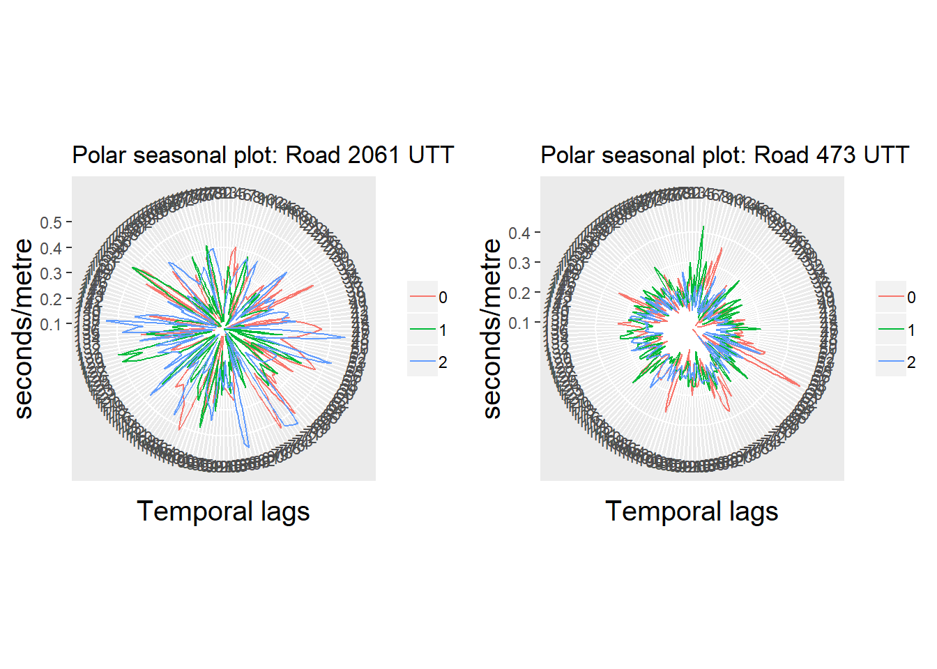
Figure 3.2: Polar seasonal plots: UTT time series (3 first days) of links with higher variation
Next, we will apply the STL decomposition for the 23 days time series. The STL() function of stats package decomposes the time series into seasonal, trend and irregular components using loess.8
Initially, the default values of the parameters are used, where the span in lags of the loess window for seasonal extraction, function s.window(), is periodic and for the trend extraction function t.window() is defined by (1.5*period) / (1-(1.5/s.window).
Here, we will select two road links: 2112 and 473.
ts_train_2112 <- ts_roadLink.2112
ts_test_2112 <- ts_test.2112
ts_train_473 <- ts_roadLink.473
ts_test_473 <- ts_test.473

ts_train_2112 %>% stl(s.window = "periodic") %>%
  autoplot() +
  xlab("Day") +
  theme(text = element_text(size = 15)) +
  ggtitle("Seasonal Decomposition: Road Link 2112 UTT")
Figure 3.3: STL decomposition for time series
ts_train_473 %>% stl(s.window = "periodic") %>%
  autoplot() +
  xlab("Day") +
  theme(text = element_text(size = 15)) +
  ggtitle("Seasonal Decomposition: Road Link 473 UTT")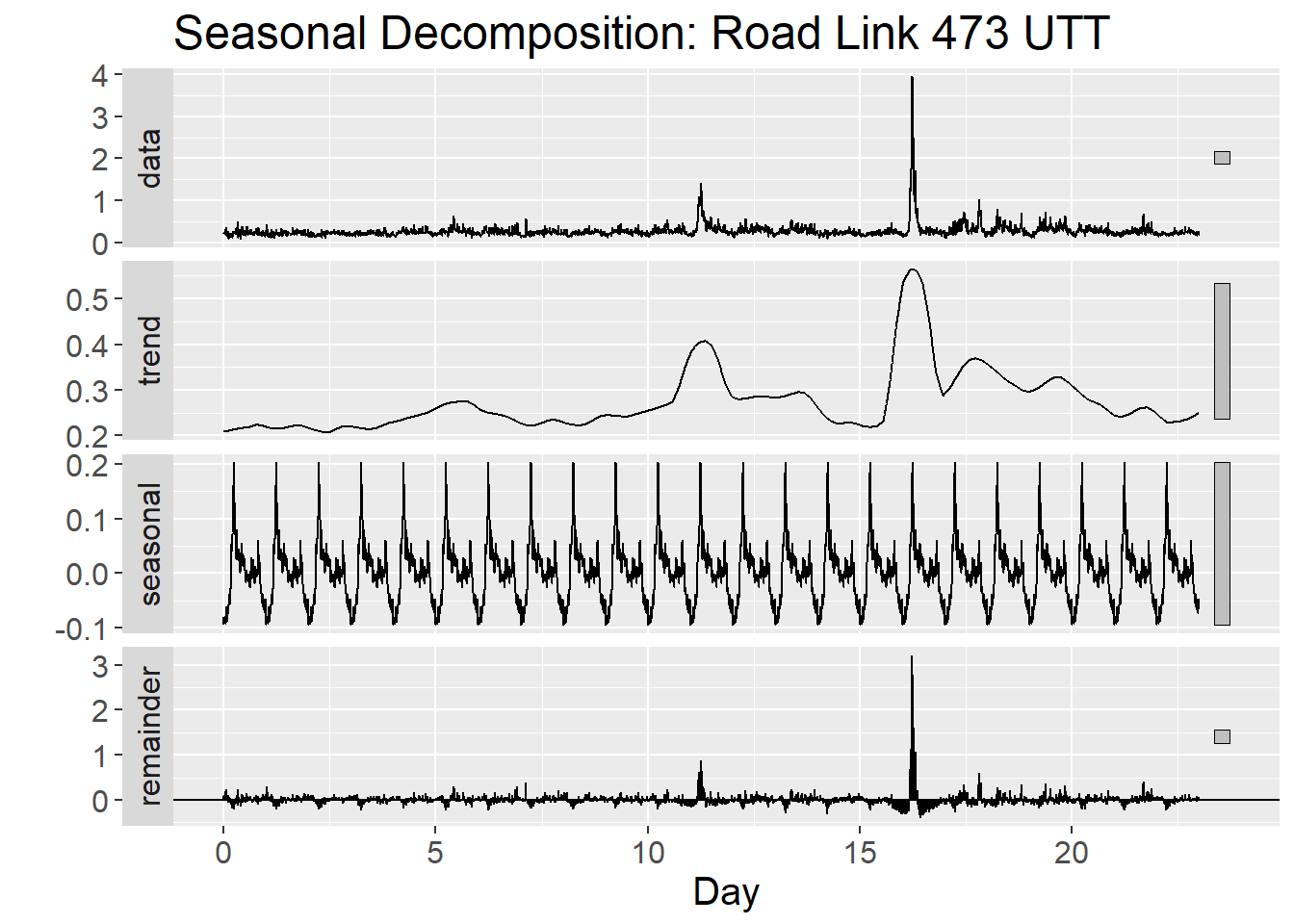
Figure 3.4: STL decomposition for time series
The STLF() function of the forecast package in R runs the STL and ETS approaches with the following default parameters:
stlf(y, h = frequency(x) * 2, s.window = 13, t.window = NULL, robust = FALSE, lambda = NULL, biasadj = FALSE, x = y, ...)`Some additional parameters are included here:
h(): number of lags or periods for forecastingrobust(): IfTRUE, robust fitting will used in the loess procedure within STLlambda(): box-Cox transformation parameter. There will be no transformation if it is equal toNULL. Otherwise, the forecasts are back-transformed via an inverse Box-Cox transformation (Hyndman and Athanasopoulos 2018). If set toauto, a transformation value is selected using theBoxCox.lambda()functionbiasadj(): use adjusted back-transformed mean for Box-Cox transformations. If transformed data is used to produce forecasts and fitted values, a regular back transformation will result in median forecasts. Ifbiasadj()isTRUE, an adjustment will be made to produce mean forecasts and fitted values9
Additional parameters are specified in the documentation of the R package. For this study we will set the following parameters:
h =1260(7 days from 6 am to 9 pm)s.window = “periodic
f_stl_2112 = stlf(ts_train_2112, h=1260,
             s.window = "periodic", lambda = NULL)

f_stl_473 = stlf(ts_train_473, h=1260,
             s.window = "periodic")

p1 <- autoplot(f_stl_2112) + xlab("Day") + ylab("Road link 2112 UTT")
p1 <- p1 + theme(text = element_text(size = 15))
p2 <- autoplot(f_stl_473) + xlab("Day") + ylab("Road link 473 UTT")
p2 <- p2 + theme(text = element_text(size = 15))

# plot the graphs
grid.draw(rbind(ggplotGrob(p1),
                ggplotGrob(p2),
size = "last")) 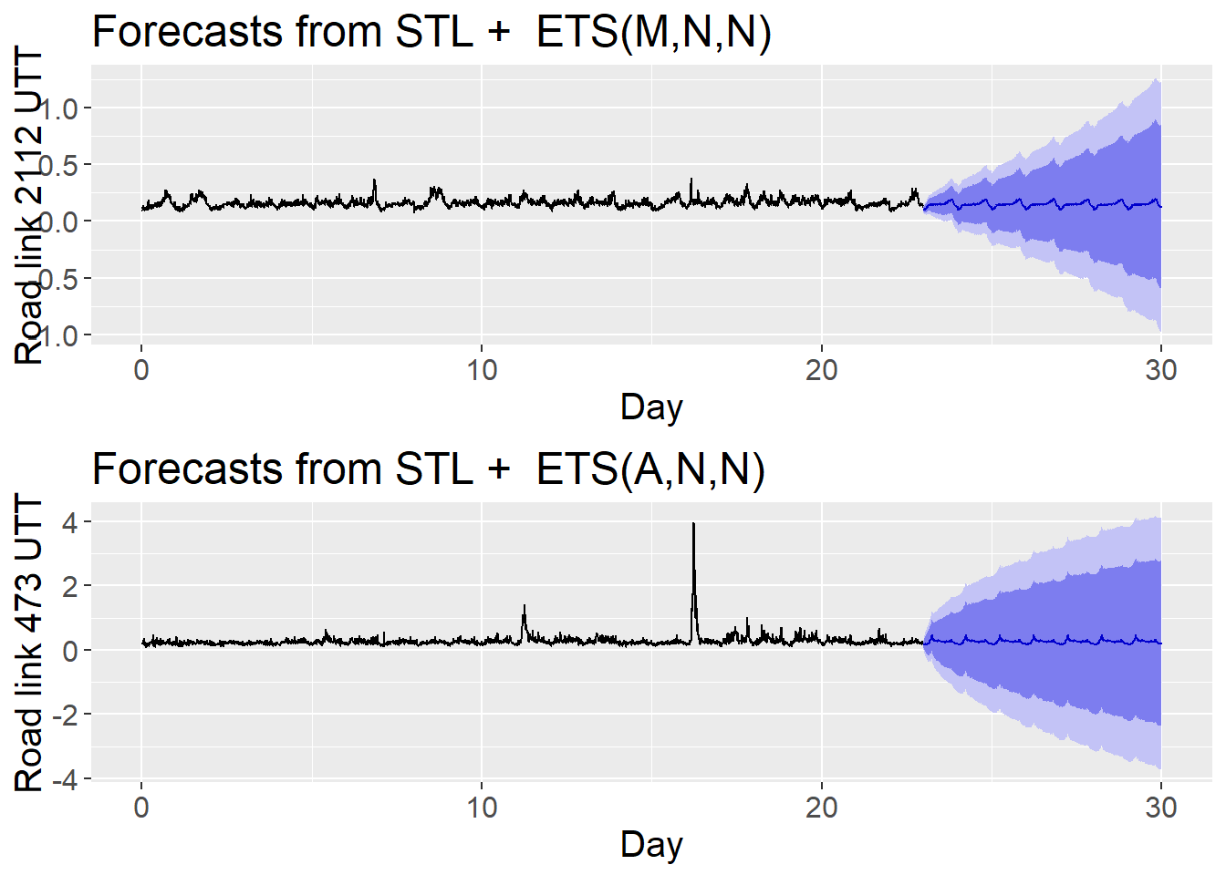
Figure 3.5: Initial STLF UTT prediction for the next 7 days
From figure 3.5, it can be observed that as the model predicts UTT values several steps ahead uncertainty increases. Thus, the interpretation of the forecasts can be significantly misleading if this uncertainty is not accounted for. To be noticed as well, road link 473 presents additive error, whereas road link 2112 presents multiplicative errors.
The following figure shows the diagnostic checking of the residuals for road link 2112 and 473. It can be observed that the residuals are normally distributed. However, some of the residuals are correlated meaning that there is more information in the errors that STLF has not accounted for.
checkresiduals(f_stl_2112)## Warning in checkresiduals(f_stl_2112): The fitted degrees of freedom is
## based on the model used for the seasonally adjusted data.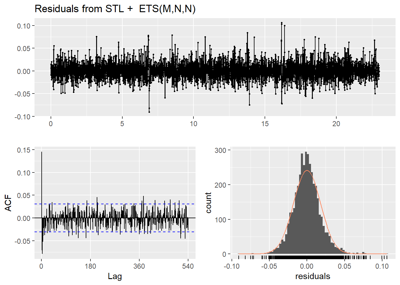
Figure 3.6: Residuals from STLF model applied to the time series
##
##  Ljung-Box test
##
## data:  Residuals from STL +  ETS(M,N,N)
## Q* = 606.21, df = 358, p-value = 4.663e-15
##
## Model df: 2.   Total lags used: 360
# If the residuals are not normally distributed and uncorrelated then there is more information in the errors that has not been accounted for in the model.
# plot predictions vs obs
predicted <- f_stl_2112[["mean"]]
observed <- ts_test_2112
checkresiduals(f_stl_473)## Warning in checkresiduals(f_stl_473): The fitted degrees of freedom is
## based on the model used for the seasonally adjusted data.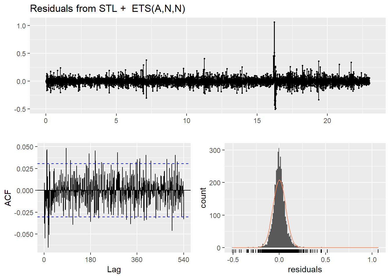
Figure 3.7: Residuals from STLF model applied to the time series
##
##  Ljung-Box test
##
## data:  Residuals from STL +  ETS(A,N,N)
## Q* = 480.28, df = 358, p-value = 1.606e-05
##
## Model df: 2.   Total lags used: 360
# If the residuals are not normally distributed and uncorrelated then
# there is more information in the errors that has not been accounted for in the model.
# plot predictions vs obs
predicted <- f_stl_473[["mean"]]
observed <- ts_test_473We can use the model for one-step-ahead prediction and plot the results, which are shown in figure 3.8. The graph shows the plots of the predicted UTT for road link 2112 and the observed or real values.
predicted <- f_stl_2112[["mean"]]
observed <- ts_test_2112

# Simple plot
plot(observed, col = "blue", xlab = "Days", ylab="UTT")
lines(predicted, col="red",lty=2)
legend(23,max(observed),legend=c("Observed","Predicted"), col=c("blue","red"),lty=c(1,2), ncol=1)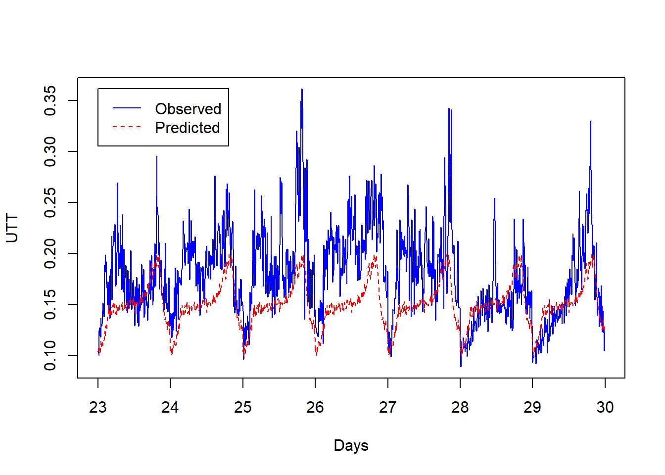
Figure 3.8: Observed and predicted values of UTT for road link 2112
We can finally print the measurements of performance of our experiment.
accuracy(predicted, observed)## ME RMSE MAE MPE MAPE ACF1
## Test set 0.02958335 0.04571804 0.03563482 13.4773 18.05772 0.7540641
## Theil's U
## Test set 1.660111Where:
- ME: Mean Error
- RMSE: Root Mean Squared Error
- MAE: Mean Absolute Error
- MPE: Mean Percentage Error
- MAPE: Mean Absolute Percentage Error
- MASE: Mean Absolute Scaled Error The first 5 are traditional measurements of forecast accuracy or performance.
MASE was introduced by Hyndman who suggested that it should become the standard metric for comparing forecast accuracy across multiple time series, where the forecast error is scaled by the in-sample mean absolute error obtained using the naïve forecasting method (Hyndman and Athanasopoulos 2018). MASE values greater than 1 show the forecasts are poorer than one-step forecasts from the naïve method.10
3.4 Chapter Summary
Time series decomposition involves thinking of a series as a combination of level, trend, seasonality and noise components. Decomposition provides a useful abstract model for thinking about time series generally and for better understanding problems during time series analysis and forecasting.
Seasonal and Trend Decomposition with Loess Forecasting Model is a versatile and robust method for decomposing time series. The model presents several advantages over other methods:
STLF can handle any type of seasonality, not only monthly and quarterly data
The seasonal component is allowed to change over time, and the rate of change can be controlled by the user
The smoothness of the trend-cycle can also be controlled by the user
It can be robust to outliers, that is the user can specify a robust decomposition so that occasional unusual observations will not affect the estimates of the trend-cycle and seasonal components. They will, however, affect the remainder component.
References
Cleveland, Cleveland, R. B., and I. Terpenning. 1990. “STL: A Seasonal Trend Decomposition Procedure Based on Loess.” Journal of Cleaner Production 6: 3–73.
Holt, C. C. 2004. “Forecasting Seasonals and Trends by Exponentially Weighted Moving Averages.” International Journal of Forecasting 20(1): 5–10.
Hyndman, R. J., and G. Athanasopoulos. 2018. Forecasting: Principles and Practice. OTexts.
The documentation of
STL()is available in: https://www.rdocumentation.org/packages/stats/versions/3.6.0/topics/stl↩Full documentation of
forecastis available in: https://www.rdocumentation.org/packages/stats/versions/3.6.0/topics/stl↩With naïve forecasts, we simply set all forecasts to be the value of the last observation.↩